Diciembre de 2020
DYNAMICAL SYSTEM ANALYSIS APPROACH TO CLIMATE AND CLIMATIC CHANGE ON VERACRUZ, MÉXICOWalter Ritter Ortiz, Lorena Cruz

Sección de Bioclimatología, Centro de Ciencias de la Atmósfera, UNAM. Circuito interior s/n, Ciudad Universitaria, Deleg. Coyoacan, México, D. F. email: walter@atmosfera.unam.mx .
Abstract
Model building admits a variety of broadly different approaches. System analysis at one end of this model spectrum, strives for detailed and pragmatic descriptions of quite specific systems. At the opposite end of the spectrum is a strategic approach, which sacrifices precision in an effort to grasp general principles. This presentation focuses on understanding the distribution of precipitation in both space and time. Temporal time series and frequency power spectra of local neighboring precipitation are described by the logistic equation which is commonly used in ecological studies. The description of precipitation spectra in terms of the logistic equation more clearly shows the underlying chaotic nature of local precipitation patterns. Intervals in the forecast of rainfall tendencies start with the signs of the critical value of the dominant maximum eigenvalue in the dynamic and future tendencies of the system. On this basis we treat the relationship between the dynamic of climatic models in which all environmental parameters are strictly deterministic, and the corresponding more realistic models with random environmental fluctuations. The calculus of precipitation tendencies determined by this methodology in the coastal State of Veracruz, México, has proved to be correct in over 85% of the total values considered.
Climatological observation stations have registered a higher percentage of unstable behavior tendencies in dryer arid regions with short range periodicities, while more stable tendencies are observed in more productive regions or those with higher levels of precipitation that show near decadal periodicities. In the area, the higher the latitudes and the aridity values the less stable the systems are, which tend to become unstable producing even shorter range periodicities. Similar conditions are observed in areas with complex orographies and strong winds, which act as perturbing external random systems, producing the total disappearance of significativies periodicities. Also, the presence of El Niño is generally manifested with the appearance of a logistic route to chaos behavior.
Key words: system analysis, climate and climate changes, chaos, precipitation.
INTRODUCTION
Nature is complex: however there is a strong trend to build simple mathematical models of the real world with the hope of grasping the essential patterns and observed processes. This approach has enjoyed considerable success in the field of ecology. Today there are an increasing number of models in climatology and climate change. The debate centers over their usefulness since they show astonishing properties as simplified deterministic models which allow extremely complicated forms of behavior. One of these models is the logistic one which considers the essential characteristics of precipitation B in a limited environment which is usually expressed as Where the relative growth rate takes the form being positive when the precipitation (B) is less than the saturation annual accumulative values for the area, known also as carrying capacity (K) and being negative when precipitation is above the K value. Stable global equilibrium is reached in the case B* = K.
Specific form of these equations are representatives of a wide group of non-linear equations having regulatory mechanisms acting exclusively on the saturation K value of the system, in addition of the intrinsic rate of growth for the time of rainy season (r) or time to reach the saturation value. In this fashion and by successive bifurcations an infinite ranking of stable cycles on rain is produced having a period 2n and converging to a limit value rc after which the system enters into a chaotic regime. Such bifurcations called a “route to chaos” can cascade into an increasing complexity of dynamic patterns, predicted by a mathematical logistic model and on precipitation data designed to test the occurrence of these bifurcations. We will become involved with deterministic a stochastic modelling parameter estimation and model validation, stability and unstability of dynamic attractors. Where to associate observations of data with mathematical predictions, requires a strong connection between models and data, where a low dimensional deterministic model can provide accurate descriptions and predictions of the complex dynamics.
In this case arbitrarily chosen close initial condition may lead after a while to widely diverging trajectories. It is for this reason that once placed in the chaotic zone the dynamic of deterministic models is better described in probabilistic terms. [1, 2, 3, 4, 5].
In high dimension cases eigenvalues can be complex and there exist other possibilities. Higher dimensional models can also display other types of bifurcations and other sequences, where the route to chaos is not of the period-doubling type, which can be determined by using methods in stability theory, where the periodic cycles and their stability is a fixed point of its initial state of the recursion formula applied n times. [6, 7, 8]. For complicated attractors analysis is best carried out in phase space where they may be considerable easier to discern, [ 9, 10].
When hazardous variations occur unidimensionally in r, we may say that has a log normal distribution. In order to solve the equation for K, Bt is dependent of a harmonic mean weight for K’s, in which r indicates how fast the former K values are mitigated, [11, 12].
An environment displaying fluctuations affects r or k or both. When both parameters vary, we have
For a predictable environment, that is auto-correlation between successive K values exists, and considering that the carrying capacity (or saturation capacity) may be represented as a first order autoregressive process; we have
The carrying capacity at t, is ? times the value at t-1 plus an independent random component Zt (with a mean zero value and variance). Under this condition ? is, in addition of controlling Kt predictability, is a measure of speed of the resource recuperation.
If ? is positive the effect of Kt-1 persists in Kt and then the autocorrelation shall be given by where -1
If ? is negative it indicates an oscillatory environment while fluctuates between positive and negative signs. A high value for ? when <, means a slow resource recovery.
On the contrary when exceeds this is an indication of high persistence of additional precipitation resources.
If the environment is completely unpredictable ?=0 and
Thus precipitation variability and predictability is determined simultaneously by its own dynamic of rainy season duration (r) and by that of the environment (?) which relates its cumulative annual values in the historic time, [13, 14, 15, 16, 17,18, 19, 20, 21].
For the deterministic case if the point of stable equilibrium of precipitation is altered, we have for small alterations the dynamics is described by the Jacobian matrix and the characteristic time required to return to equilibrium is measured by the real part of the eigenvalues. In a stochastic environment, there exist a wide range of possible values of precipitation as described by the equilibrium probabilistic distribution function in which in addition there exists a continuous spectrum of disturbances, generated by the stochasticity of the external environment.
While the internal dynamics of precipitation interactions tends to restore it to its saturation mean value, (that is to say to compact the cluster of precipitation values) the random fluctuations of the external environment act in order to disperse them, [4, 5,13].
One relevant aspect of external environmental fluctuation is the drought phenomenon. However, even in the case of the absence of drought, precipitation will vary in amount with respect to the one obtained under constant external conditions. As a result the magnitude of precipitation may reach different values and what is of interest is the probabilistic distribution of the presence of such values.
METHODOLOGY
The logistic equation used in this project possesses the property that one of its parameters known as “the intrinsic rate of growth” (r) determines the dynamics of the system. The stability of these equations can be proved through calculus; however it can be done geometrically as well, by means of diagrams of graphical methods of iteration, [19]. When r is smaller that 3, the curve of the equation obtains its stability rotating inwards in spiral; however, if r is greater than 3, it will rotate outwards in spiral conforming an unstable static point, Figure (1). Hence, if r passes from Zero to 4, it gains a regular increase in the complexity of the dynamic behaviour: going from a stationary value towards a periodic and from there to a chaotic one, [4, 5].
Following methodologies proposed by [11] the values of r are calculated constructing the graphics of Ln(K-B(t))/B(t) against time t, figure(2) in which K is obtained in the graphics of the annual accumulative rainfall in the areas of saturation. Observe that in these graphics we find the situation of a variable K with more than one or two values. Also, in the calculus of the values of r, some of the values remain outside the expected range, which can be considered to be extreme events or resultants of random external effects in the system. The forecasting discrete logistic equations is given by; X(t+1)= rX(t)(1-X(t)), where X=B/K.
RESULTS
The system of precipitation time series analysed as a dynamic system (exponent of positive Lyapunov and dimension of low order), indicates that in Veracruz, México, figure(3) the rainfall system is chaotic, and for that reason, it is predictable in the short range.
The logistic model can be identified and shown capable of not only accurate fitting of data, but also accurate predictions of data, figure(2).
- In the State of Veracruz, precipitation vectors in space phases, invading the chaotic zone, corresponding to the maximum eigenvalue derived from the Jacobian of the logistic equations, are responsible of determining the predictive dynamic of the system, where we observe that through the sign of this eigenvalue we can not only determine tendencies, but also future values in the abundance of regional precipitations. The tendency to positive eigenvalues correspond to abundant rainfall, and the tendency to negative eigenvalues, to the occurrence of drought situations, as has been pointed out by [18, 19, 20, 21] on the productivity ecosystems, figure (4).
The calculus of precipitation tendencies determined by this methodology in the coastal State of Veracruz has proved to be correct in over 85% of the total values considered.
Intervals in the forecast of rainfall tendencies start with the critical value of the eigenvalue vector that invades the “chaotic area”, and ends up when a new invading vector is introduced in the same area, which will become the new dominant maximum eigenvalue in the dynamic and future tendencies of the system, figures (4, 5).
-In certain occasions, precipitation vectors in the space phase graphs tend to over-stimulate the system, withdrawing from the basic attractor through the performance of unstable repulsive outwards and attracting stable inwards turns that tend to become predictable in the dynamic of the logistic equation, figure (4).
Climatological observation stations indicate a higher percentage of unstable tendencies in the Northern dry arid regions of the State while stable tendencies in the Southern more productive regions or those with higher levels of precipitation, figure (1). Such conditions have already been observed by [16, 17], in a comparative rainfall analysis carried out in various areas of the country.
External aleatory effects in the rainfall system in the State of Veracruz, such as strong winds (widely known in some areas) along with the orography itself act as filters in the presence of possible decadal periodicities in the historical precipitation data, figure (3).
The presence of El Niño is generally manifested also with the appearance of a chaotic behaviour, through a logistic route to chaos, which can be observed in the graphics presented by [19, 22].
Aknowledgments
We would like to express our gratitude to Alfonso Salas Cruz and Rafael Patiño Mercado for their support during the process of this document.
Bibliography
[1]May R.M.(1974) Biological populations with nonoverlapping generations: points, stable cycles and chaos, Science 186, 645-647.
[2]May R.M. (1976) Simple mathematical models with very complicated dynamics, Nature 261, 459-467.
[3]May R.M. and G.F. Oster(1976) Bifurcations and dynamic complexity in simple ecological models, The American Naturalist 110, 573-599.
[4]May R.M. (2001) Stability and Complexity in model Ecosystems, Princeton Landmarks in Biology, Princeton University Press, Princeton, NJ.
[5]Lee T.Y. and Yorke (1975) Period three implies chaos, American Mathematical Monthly 82, 985-992.
[6]Kareiva P. (1995) Predicting and producing chaos, Nature 375, 189-190.
[7]Guckenheimer J. and P. Holmes(1983) Nonlinear Oscillations, Dynamical Systems and Bifurcations of Vector Fields. Springer-Verlag, Berlin.
[8]Auyang S.Y.(1998) Foundations of complex system Theories in Economics, Evolutionary Biology and Statistical Physics. Cambridge University Press. Cambridge, UK
[9]Pool R.(1989) It is chaos, or is it just noise?. Science 243, 25-28.
[10]Ellner S.and P. Turchin(1995) Chaos in a noisy world: new methods and evidence from time-series analyses, The American Naturalist 145, 343-375.
[11]Vandermeer J. H. (1972) Elementary Mathematical Ecology. John Wiley. New York.
[12]Roughgarden, J. (1974) Population Dynamics spatialy varying environments. How population size tracks spatial variation in carrying capacity. The American Naturalist. Vol.108, No. 963.
[13]Seber G.A.F.(1984) Multivariate Observations, Jhon Wiley&Sons, New York
[14]Sugihara G., and R. M. May (1990) Nonlinear forecasting as a way of distinguishing chaos from measurement error in time series, Nature 344(1990), 734-741.
[15]Ritter O. W., A. Noguez y I. Rosas (1988) Evaluation of agriculture stability production from climatic indices, for some Mexican localities. Geofisica Internacional, 7 (2), 263-278 (in Spanish)
[16]Ritter O.,W., Mosiño P., A., Buendía C., E. (1998)” Dynamic Rain Model for Lineal Stochastic Environments”. Quaterly Journal of Meteorology (India)(Mausam), Vol. 49,No.1. Pp. 127-134.
[17]Ritter O. W., Jauregui O. E., Guzman R. S., Estrada B. A., Muñoz N. H., Suarez S. J. and Corona V. MC.(2004) Ecological and agricultural productivity indices and their dynamics in a sub-humid/semi-arid region from Central México. Journal of Arid Environments 59, 753-769.
[18] Ritter O. W., Suárez S. J., (2005). Predictability and phase space relationships of climatic changes and tuna biomass on the Eastern Pacific Ocean. 6 eme Europeen de Science des Systemes Res-Systemica volume no. 5, Special Issue. FRANCE.
[19]Ritter O. W., Suarez S. J.(2011) Impact of ENSO and the optimum use of yellowfin tuna in the Easthern Pacific Ocean Region. Ingenieria de Recursos Naturales y del Ambiente, numero !9, enero-diciembre, 2011, pp. 109-116, Universidad del Valle, Cali Colombia.
[20]Suarez S.J., W. O. Ritter, C. G. Gay, J Torres Jacome (2004) ENSO- Tuna- relations in the eastern Pacific Ocean and its prediction as a non-linear dynamic system. Atmósfera, pags. 245-258.
[21]Seber G.A.F.(1984) Multivariate Observations, Jhon Wiley&Sons, New York
[22]Vandermeer J. H. (1972) Elementary Mathematical Ecology. John Wiley. New York.
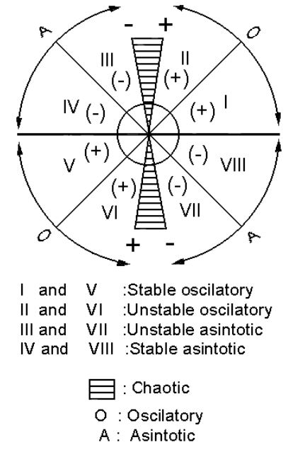
figure 1 Graphic method modified by Ritter et al (2004) in order to calculate phase space eigenvalues as well as the system’s behavioural patterns divided in a: oscillatory, asymptotic, stable or unstable and chaotic area.
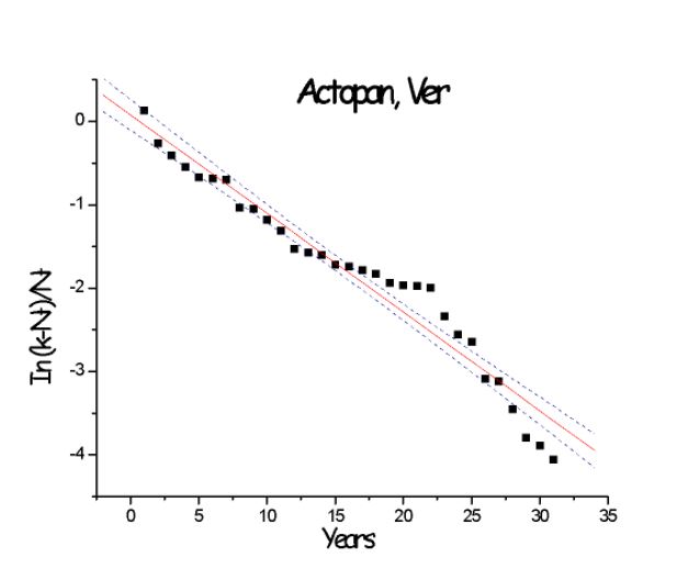
Figure 2.- Adjustment of precipitation values to logistic equation in order to determine simulation and prognosis coefficients
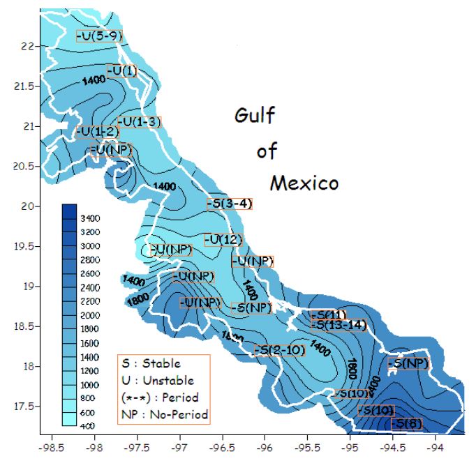
Figure 3.- Mean distribution of isohyets (mm/year) for the state of Veracruz for period 1940-2000. Space/dynamic behaviour of stable(S)/unstable(U) conditions and significant periodicities(in parenthesis). (NP) means non-significant periods.
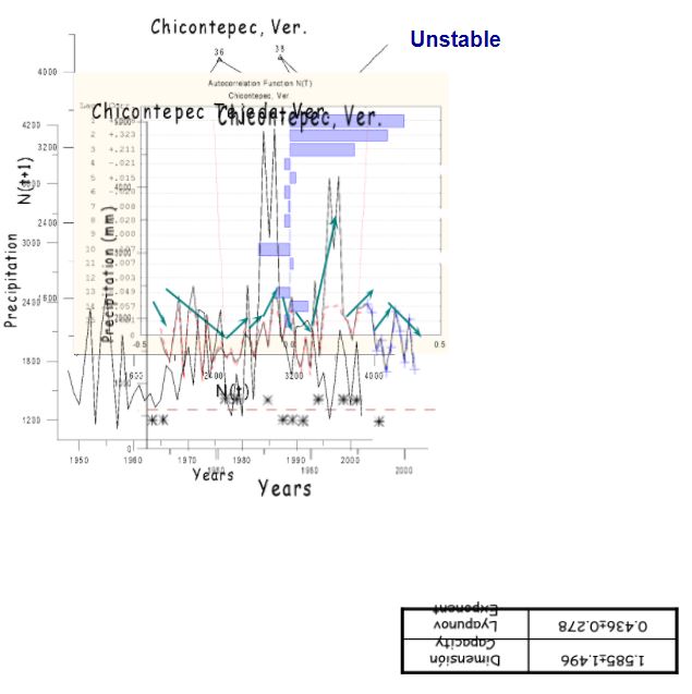
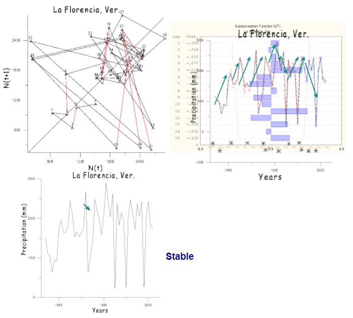
Figure 4.- Phase-space of a system with stable/unstable dynamics and corresponding capacity dimension values as well as Lyapunov exponents and autocorrelations, annual precipitation values and their maximum eigenvalues in which positive values correspond to excessive precipitation trends while those negative correspond to deficient trends.
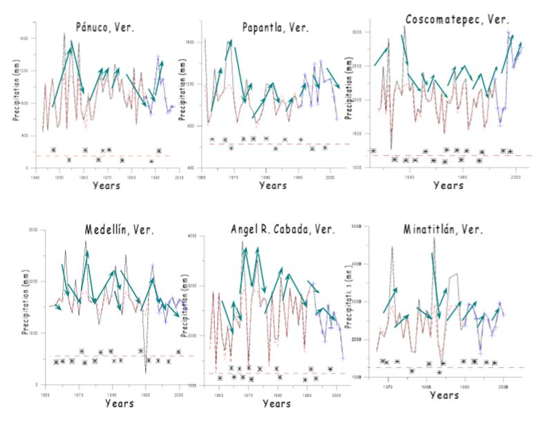
Figure 5.- Mean annual precipitation values observed at 6 regions of the Veracruz state and their corresponding prognostic values derived from the logistic equation, in which difference spaces point to those random effects of environmental external noise.
 Visitas: 1108